Normal distribution, binomial distribution, and Poisson distribution are three important probability distributions used in statistics and data analysis.

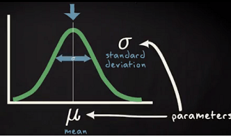
The normal distribution, also known as the Gaussian distribution, is a continuous probability distribution that is often used to describe natural phenomena such as heights and weights. It is characterized by its bell-shaped curve, which is symmetric and centered around the mean. The standard deviation determines the width of the curve and describes the variability of the data.

The binomial distribution is a discrete probability distribution that is used to model the number of successes in a fixed number of independent trials. It is characterized by two parameters – the probability of success in a single trial, and the number of trials. The binomial distribution is widely used in fields such as finance, biology, and quality control.

The Poisson distribution is a discrete probability distribution that is used to model the number of events that occur in a fixed interval of time. It is characterized by a single parameter – the average number of events per unit time. The Poisson distribution is often used in fields such as epidemiology, finance, and telecommunications.

Normal Distribution or Gaussian Distribution or Bell Curve 

In probability theory, the normal distribution or Gaussian distribution is a very common continuous probability distribution. The normal distribution is sometimes informally called the bell curve.

The probability density of the normal distribution is:

 is mean or expectation of the distribution

 is the variance

In short hand notation of normal distribution has given below.

Cumulative normal probability distribution will look like the below diagram.

Properties of a normal distribution

• The mean, mode and median are all equal.
• The curve is symmetric at the center (i.e. around the mean, μ).
• Exactly half of the values are to the left of center and exactly half the values are to the right.
• The total area under the curve is 1.

Normal Distribution Probability Calculation

Probability density function or p.d.f. specified the probability per unit of the random variable. Here is an example of a p.d.f. of the daily waiting time by the taxi driver of Uber taxi company. In the X axis, daily waiting time and Y-axis probability per hour has been shown.

 

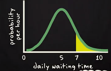
If one Uber taxi driver want to know the probability to wait more than 7 hours in a day?

Then he will be interested in the yellow surface arear shown above. On basis of this graph you can estimate the area. Same thing you can get form below cumulative probability curve.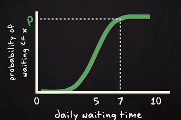

Probability to wait more than 7 hours will be calculated using complementary rule 1- P. Because corresponding to 7 in X axis we marked the probability is P and we are interested in more than 7 hours. So, P should be subtracted from 1 to get desired result.

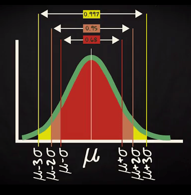
Bell Shaped Distribution and Empirical Rule

If distribution is bell shape then it is assumed that about 68% of the elements have a z-score between -1 and 1; about 95% have a z-score between -2 and 2; and about 99% have a z-score between -3 and 3.

Assume the time you spend in week days by traveling has given by a normal distribution with mean= 40 mins and SD= 10 mins.

What will be your range of travel time for 95 % of your week days?

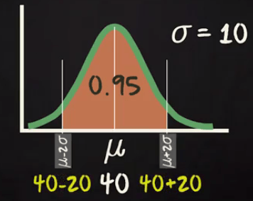
As you know 95 % will come within 2 standard deviation of your mean. So, the range will be (40-20) = 20 to (40+20) =60 mins.

Now, another question you want to answer that what will be the probability to be travelling more than 50 mins?

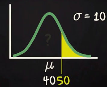
Actually, you are interested in the yellow surface given in above diagram. You know that a normal distribution is symmetric. So, half of the probability located one side of the mean and another half located another side of the mean.

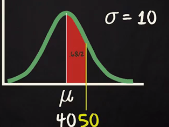
As SD =10. So, one standard deviation will be 30 to 50 range.

You already know for left side up 40 the probability is 0.5. Now if you calculate the probability from 40 to 50 range it will be half of 1 Standard deviation i.e.    0.68/2 = 0.34

So the probability to travel less than 50 mins = 0.5 +. 0.34 = 0.84

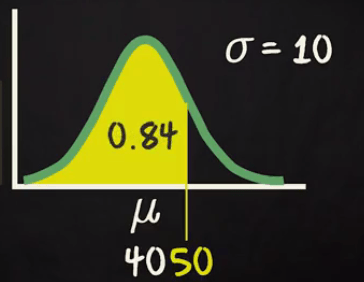
But you are interested in more than 50 mins traveling time so it will be 1- 0.84 =0.16

Bernoulli trial & Binomial Distribution

Every random variable has a corresponding probability distribution. The probability distribution applies the theory of probability to describe the behavior of the random variable. A discrete random variable X has a finite number of possible integer values. The probability distribution of X lists the values and their probabilities in a table

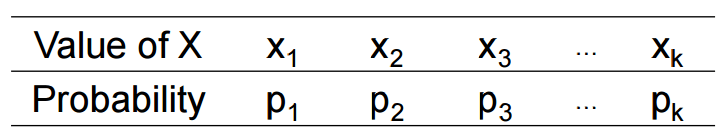
• Every probability pi is a number between 0 and 1.
• The sum of the probabilities must be 1.

This properties we have already studied before. Now we will discuss about the most important probability for discrete random variable is Binomial Distribution. Before that it is necessary to know about Bernoulli trial.

Bernoulli trial or Binomial Trial

Bernoulli trial (or binomial trial) is a random experiment with exactly two possible outcomes, “success” and “failure”, in which the probability of success is the same every time the experiment is conducted.

• The event (or trial) results in only one of two mutually exclusive outcomes – success/failure
• Probability of success is known, P(success) = π

Bernoulli trial or Binomial Trial Examples

– A single coin toss (heads or tails), P(heads) = π = 0.5

– Survival of an individual after CABG surgery, P(survival) = π = 0.98

– Pick an individual from the Indian population, P(obese) = π = 0.31

Binomial Distribution

A distribution is said to be binomial distribution if the following conditions are met.

1. Each trial has a binary outcome (One of the two outcomes is labeled a ‘success’)
2. The probability of success is known and constant over all trials
3. The number of trials is specified
4. The trials are independent. That is, the outcome from one trial doesn’t affect the outcome of successive trials

If all the above conditions met then the binomial distribution describes the probability of X successes in n trials.



A classic example of the binomial distribution is the number of heads (X) in n coin tosses.

The Notation for a binomial distribution is

X ~ B (n, π)

which is read as ‘X is distributed binomial with n trials and probability of success in one trial equal to π ’.

Formula for Binomial Distribution

Using this formula, the probability distribution of a binomial random variable X can be calculated if n and π are known.

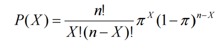
n! is called ‘n factorial’ = n(n-1)(n-2) . . .(1)

P(X) = #of Scenario * Single Scenario

The first factorial terms gives the number of scenario and the second term describes the probability of success to power of number of successes and probability of failure to the power of number of failures.

Binomial Distribution Example

What is the probability of 2 heads in 6 coin tosses?

• Success = ‘heads’
• n = 6 trials
• π = 0.5
• X = number of heads in 6 tosses which is 2 here.
• X has a binomial distribution with n = 6 and π = 0.5
• X ~ B (6, 0.5)

So, probability of getting 2 heads is 0.234.

Consider another example:

In a sample of 8 patients with a heart attack, what is the probability that 2 patients will die if the probability of death from a heart attack = 0.03.

Assume that the probability of death is the same for all patients.

– Death from heart attack is a binary variable (Yes or No)

– ‘Success’ in this case is defined as death from heart attack

– n = number of ‘trials’ = 8 patients

– π = 0.03 = probability of success

– X = number of deaths. X =2 here.

X ~ B (8, 0.03)

If you follow the same formula you will get P(x=2) = 0.021

Poisson Distribution

Another probability distribution for discrete variables is the Poisson distribution. The Poisson distribution is used to determine the probability of the number of events occurring over a specified time or space. This was named for Simeon D. Poisson, 1781 – 1840, French mathematician.

Examples of events over space or time: -number of cells in a specified volume of fluid

-number of calls/hour to a help line

-number of emergency room beds filled/ 24 hours

Like the binomial distribution and the normal distribution, there are many Poisson distributions.

• Each Poisson distribution is specified by the average rate at which the event occurs.
• The rate is notated with λ
•  λ = ‘lambda’, Greek letter ‘L’ – There is only one parameter for the Poisson distribution

The probability that there are exactly X occurrences in the specified space or time is equal to

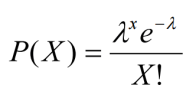
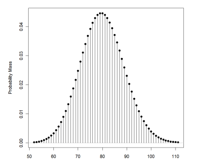
The horizontal axis is the index X. The function is defined only at integer values of X. The connecting lines are only guides for the eye and do not indicate continuity. Notice that as λ increases the distribution begins to resemble a normal distribution.

• If λ is 10 or greater, the normal distribution is a reasonable approximation to the Poisson distribution
• The mean and variance for a Poisson distribution are the same and are both equal to λ
• The standard deviation of the Poisson distribution is the square root of λ

Poisson Distribution Example

A large urban hospital has, on average, 80 emergency department admits every Monday. What is the probability that there will be more than 100?

If we put λ =80 and  x= 100 then we will get the probability value as 0.01316885.

To get the same result we can use normal approximation and then get the probability value.

emergency room admits on a Monday?

• λ is the rate of admits / day on Monday = 80
• we can use the normal approximation since λ > 10

The normal approximation has mean = 80 and SD = 8.94 (the square root of 80 = 8.94)

Now, we can use the same way we calculate p-value for normal distribution. If you do that you will get a value of 0.01263871 which is very near to 0.01316885 what we get directly form Poisson formula. Here main intention is to show you how normal approximation works for Poisson Distribution.

Understanding these distributions and their properties is essential for many applications in fields such as finance, engineering, and science. By analyzing data using these distributions, we can make predictions and draw conclusions about real-world phenomena.